Introduction to Data Science ¶

1MS041, 2023¶

Estimating the distribution function¶

Suppose we don't know what the distribution function (DF) is? We are not trying to estimate some fixed but unknown parameter $\theta^*$ for some RV we are assuming to be $Bernoulli(\theta^*)$, we are trying to estimate the DF itself. In real life, data does not come neatly labeled "I am a realisation of a $Bernoulli$ RV", or "I am a realisation of an $Exponential$ RV": an important part of inference and estimation is to make inferences about the DF itself from our observations.

Observations from some unknown process¶

Consider the following non-parametric product experiment:

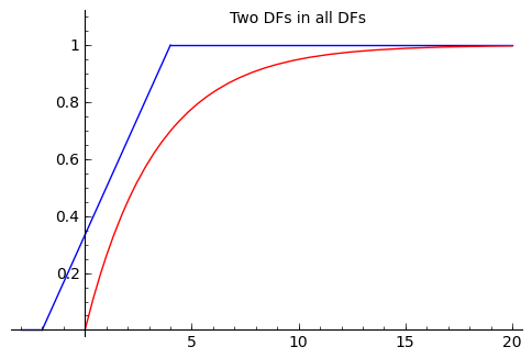
$$X_1, X_2, \ldots, X_n\ \overset{IID}{\sim} F^* \in \{\text{all DFs}\}$$

We want to produce a point estimate for $F^*$, which is a allowed to be any DF ("lives in the set of all DFs"), i.e., $F^* \in \{\text{all DFs}\}$

Crucially, $\{\text{all DFs}\}$, i.e., the set of all distribution functions over $\mathbb{R}$ is infinite dimensional.

We have already seen an estimate, made using the data, of a distribution function: the empirical or data-based distribution function (or empirical cumulative distribution function). This can be formalized as the following process of adding indicator functions of the half-lines beginning at the data points $[X_1,+\infty),[X_2,+\infty),\ldots,[X_n,+\infty)$:

$$\widehat{F}_n (x) = \frac{1}{n} \sum_{i=1}^n \mathbf{1}_{[X_i,+\infty)}(x)$$

where,

$$\mathbf{1}_{[X_i,+\infty)}(x) := \begin{cases} & 1 \quad \text{ if } X_i \leq x \\ & 0 \quad \text{ if }X_i > x \end{cases}$$

Lets take a look at this for an example

import numpy as np
X = np.random.poisson(1,size=1000)
from Utils import makeEDF, makeEMF, plotEDF
print(makeEDF(X))
plotEDF(makeEDF(X))

Dvoretsky-Kiefer-Wolfowitz (DKW) Inequality¶

Let $X_1, X_2, \ldots, X_n \overset{IID}{\sim} F^* \in \{\text{all DFs}\}$

and the empirical distribution function (EDF) is $\widehat{F}_n(x) := \displaystyle\frac{1}{n} \sum_{i=1}^n \mathbf{1}_{[X_i,+\infty)}(x)$,

then, for any $\varepsilon > 0$,

$$P\left( \sup_x { | \widehat{F}_n(x) - F^*(x) | > \varepsilon }\right) \leq 2 \exp(-2n\varepsilon^2) $$

We can use this inequality to get a $1-\alpha$ confidence band $C_n(x) := \left[\underline{C}_n(x), \overline{C}_n(x)\right]$ about our point estimate $\widehat{F}_n$ of our possibly unknown $F^*$ such that the $F^*$ is 'trapped' by the band with probability at least $1-\varepsilon$.

$$ \begin{aligned} \underline{C}_{\, n}(x) &= \max \{ \widehat{F}_n(x)-\varepsilon_n, 0 \}, \notag \\ \overline{C}_{\, n}(x) &= \min \{ \widehat{F}_n(x)+\varepsilon_n, 1 \}, \notag \\ \varepsilon_n &= \sqrt{ \frac{1}{2n} \log \left( \frac{2}{\alpha}\right)} \\ \end{aligned} $$

and

$$P\left(\underline{C}_n(x) \leq F^*(x) \leq \overline{C}_n(x)\right) \geq 1-\alpha$$

Estimating the density¶

For a discrete random variable, estimating the density (pmf) is as simple as using the empirical pmf

from Utils import plotEMF
print(makeEMF(X))
plotEMF(makeEMF(X))

For a continuous random variable¶

For a continuous random variable we cannot really use the pmf, instead we consider something like a histogram

Y = np.random.normal(size=1000)
freq,bins,_ = plt.hist(Y,density=True,bins=50)

print("     Bin \t Freq")
for frq,l_edge,r_edge in zip(freq,bins,bins[1:]):
    print("[%.2f,%.2f] \t %.2f" % (l_edge,r_edge,frq))

Whenever we want to use a histogram estimator, we need to decide how many bins we are going to need. This is a topic for another day.

Regression example of risk minimization¶

Consider the following house price data

import csv
data = []
header = []
with open('data/portland.csv', mode='r') as f:
    reader = csv.reader(f)
    header = tuple(next(reader))
    for row in reader:
        try:
            data.append((int(row[0]),int(row[1]),int(row[2])))
        except e:
            print(e)

print(header)
print(data[:1])

('Size of the house (in square feet)', 'Number of bedrooms', 'Price of the house')
[(2104, 3, 399900)]

Lets think that the data generator $X$ is here the size of the house and the $Y$ is the price of the house.

import numpy as np
D = np.array(data)
X = D[:,0]
Y = D[:,2]

import matplotlib.pyplot as plt
plt.scatter(X,Y)

<matplotlib.collections.PathCollection at 0x10f533310>

Linear regression¶

An example of a learning machine is linear regression with quadratic loss. What we have is essentially

The loss is the quadratic function
We are searching among linear functions, $g_{k,m}(x) = kx+m$.

$$ k^\ast, m^\ast = \text{argmin}_{k,m}\frac{1}{n} \sum_{i=1}^n (k X_i + m - Y_i)^2 $$

R = lambda a: np.mean(np.power((a[0]*X+a[1]-Y),2))

import scipy.optimize as so

We can use scipy to minimize the total loss $L$ above.

result = so.minimize(R,(0,0),method = 'Nelder-Mead')
result

 final_simplex: (array([[  134.52528792, 71270.49196559],
       [  134.52528791, 71270.49200697],
       [  134.52528792, 71270.49201691]]), array([4.11626548e+09, 4.11626548e+09, 4.11626548e+09]))
           fun: 4116265480.866082
       message: 'Optimization terminated successfully.'
          nfev: 330
           nit: 174
        status: 0
       success: True
             x: array([  134.52528792, 71270.49196559])

This gives us that the found $k \approx 135$ and the found $m \approx 70000$, we can also plot this together with data to see

x_pred = np.linspace(np.min(X),np.max(X),2)
y_pred = x_pred*result['x'][0]+result['x'][1]
plt.scatter(X,Y)
plt.plot(x_pred,y_pred,color='green')

[<matplotlib.lines.Line2D at 0x1112afa60>]

Introduction to Data Science¶