©2021 Raazesh Sainudiin, Benny Avelin. Attribution 4.0 International (CC BY 4.0)
data/
Here is an extract from https://en.wikipedia.org/wiki/Earthquake:
An earthquake (also known as a quake, tremor or temblor) is the shaking of the surface of the Earth resulting from a sudden release of energy in the Earth's lithosphere that creates seismic waves. Earthquakes can range in size from those that are so weak that they cannot be felt to those violent enough to propel objects and people into the air, and wreak destruction across entire cities. The seismicity, or seismic activity, of an area is the frequency, type, and size of earthquakes experienced over a period of time. The word tremor is also used for non-earthquake seismic rumbling.
At the Earth's surface, earthquakes manifest themselves by shaking and displacing or disrupting the ground. When the epicenter of a large earthquake is located offshore, the seabed may be displaced sufficiently to cause a tsunami. Earthquakes can also trigger landslides and, occasionally, volcanic activity.
In its most general sense, the word earthquake is used to describe any seismic event—whether natural or caused by humans—that generates seismic waves. Earthquakes are caused mostly by rupture of geological faults but also by other events such as volcanic activity, landslides, mine blasts, and nuclear tests. An earthquake's point of initial rupture is called its hypocenter or focus. The epicenter is the point at ground level directly above the hypocenter.
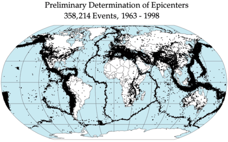
Having gotten some basic background on earthquakes (Seismologists are the domain experts of seismology or the study of earthquakes) as we will be analysing data fetched from New Zealand which is in the Ring of Fire along with Japan, Western American continental coastlines all the way down to Chile as rendered below.
Here are typical epicentres all across the globe.
def showURL(url, ht=500):
"""Return an IFrame of the url to show in notebook with height ht"""
from IPython.display import IFrame
return IFrame(url, width='95%', height=ht)
showURL('https://en.wikipedia.org/wiki/Earthquake',500)
To make the ideas sink in the following blogpost on a review of probability theory by one of the best mathematicians alive, namely Terry Tao, is highly recommended, especially for students of Mathematics.
showURL('https://terrytao.wordpress.com/2010/01/01/254a-notes-0-a-review-of-probability-theory/')
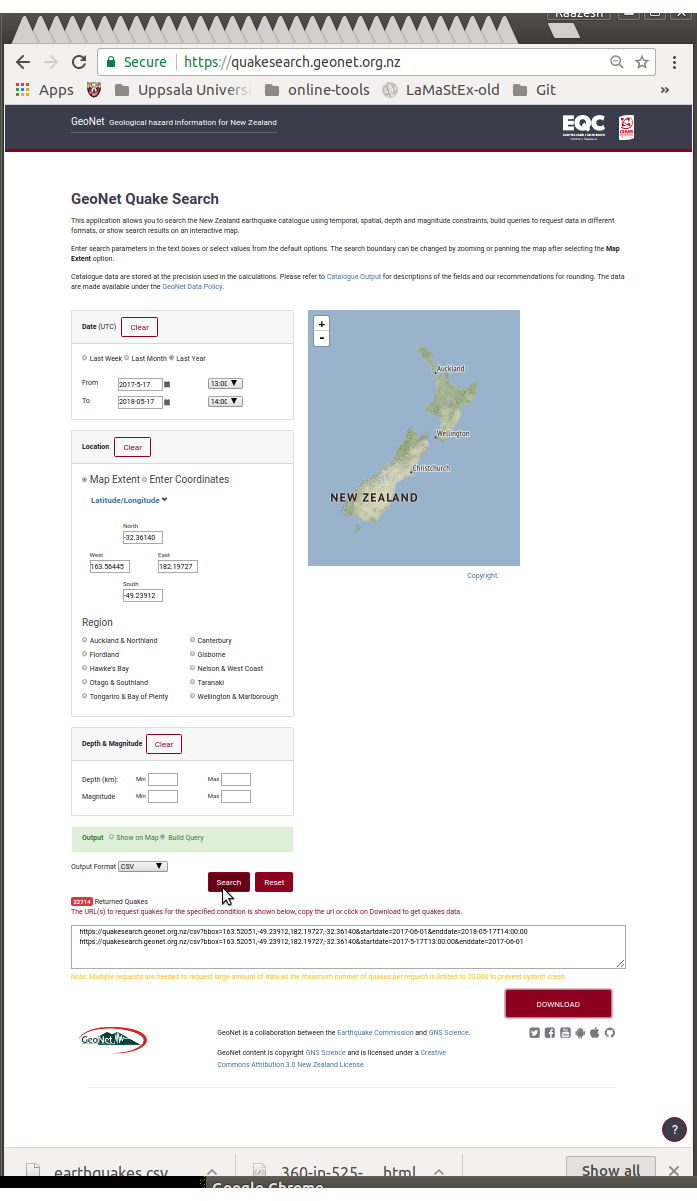
Go to https://quakesearch.geonet.org.nz/ and download data on NZ earthquakes.
In my attempt above to zoom out to include both islands of New Zealand (NZ) and get one year of data using the Last Year
button choice from this site:
Search
box gave the following URLs for downloading data. I used the DOWNLOAD
button to get my own data in Output Format CSV
as chosen earlier.https://quakesearch.geonet.org.nz/csv?bbox=163.52051,-49.23912,182.19727,-32.36140&startdate=2017-06-01&enddate=2018-05-17T14:00:00 https://quakesearch.geonet.org.nz/csv?bbox=163.52051,-49.23912,182.19727,-32.36140&startdate=2017-5-17T13:00:00&enddate=2017-06-01
Try to DOWNLOAD
your own CSV
data and store it in a file named my_earthquakes.csv
(NOTE: rename the file when you download so you don't replace the file earthquakes.csv
!) inside the folder named data
that is inside the same directory that this notebook is in.
Browser settings: Make sure you have changed your browser settings so you get asked where a downloaded file should be saved each time you download.
%%sh
### print working directory
pwd
/home/user/datascience-intro/raaz/1MS041/master/jp
%%sh
#ls ## uncomment to `ls` or list contents of working directory
%%sh
### after download you should have the following file in directory named data
ls data
CORIS.csv NYPowerBall.csv co2_mm_mlo.txt digits.csv earthquakes.csv earthquakes.csv.zip earthquakes.tgz earthquakes_small.csv final.csv final.csv.zip final.tgz leukemia.csv portland.csv pride_and_prejudice.txt rainfallInChristchurch.csv ratings.csv
%%sh
### first three lines
head -3 data/earthquakes_small.csv
publicid,eventtype,origintime,modificationtime,longitude, latitude, magnitude, depth,magnitudetype,depthtype,evaluationmethod,evaluationstatus,evaluationmode,earthmodel,usedphasecount,usedstationcount,magnitudestationcount,minimumdistance,azimuthalgap,originerror,magnitudeuncertainty 2018p371534,,2018-05-18T11:13:48.826Z,2018-05-18T11:15:55.741Z,176.469659,-38.10063545,2.123583253,93.125,M,,NonLinLoc,,automatic,nz3drx,18,18,11,0.3996779802,94.08602902,1.036195008,0 2018p371524,,2018-05-18T11:08:07.588Z,2018-05-18T11:11:14.319Z,176.4213445,-38.63584892,2.570467678,35.9375,M,,NonLinLoc,,automatic,nz3drx,22,22,11,0.3208135882,89.12864378,1.012353739,0
%%sh
### last three lines by `tail`
tail -3 data/earthquakes_small.csv
2018p352775,,2018-05-11T12:38:54.732Z,2018-05-11T12:40:28.518Z,175.6063627,-40.81585537,1.835272336,13.671875,M,,NonLinLoc,,automatic,nz3drx,22,22,12,0.1097369199,84.14006379,0.3314536834,0 2018p352725,,2018-05-11T12:12:36.343Z,2018-05-11T12:14:42.372Z,176.0372811,-38.78743116,2.103529946,76.25,M,,NonLinLoc,,automatic,nz3drx,17,17,4,0.4257033383,244.4056741,1.445270768,0 2018p352684,,2018-05-11T11:50:06.019Z,2018-05-11T11:51:41.163Z,176.5437111,-40.07042442,1.503468463,13.671875,M,,NonLinLoc,,automatic,nz3drx,13,13,7,0.079302248,81.46123042,0.4485324555,0
%%sh
### number of lines in the file; mnemonic from `man wc` is wc = word-count option=-l is for lines
wc -l data/earthquakes_small.csv
411 data/earthquakes_small.csv
#%%sh
#man wc
data/earthquakes.csv
¶This will ensure we are all looking at the same file!
But feel free to play with your own data/my_earthquakes.csv
on the side.
Grab lat, lon, magnitude
with open("data/earthquakes_small.csv") as f:
reader = f.read()
dataList = reader.split('\n')
len(dataList)
412
dataList[0]
'publicid,eventtype,origintime,modificationtime,longitude, latitude, magnitude, depth,magnitudetype,depthtype,evaluationmethod,evaluationstatus,evaluationmode,earthmodel,usedphasecount,usedstationcount,magnitudestationcount,minimumdistance,azimuthalgap,originerror,magnitudeuncertainty'
dataList[-1] ## Remember last line is empty
''
myDataAccumulatorList =[]
for data in dataList[1:-2]:
dataRow = data.split(',')
myData = [dataRow[4],dataRow[5],dataRow[6]]
myFloatData = tuple([float(x) for x in myData])
myDataAccumulatorList.append(myFloatData)
points(myDataAccumulatorList)
Recall that a statistic is any measurable function of the data: $T(x): \mathbb{X} \rightarrow \mathbb{T}$.
Thus, a statistic $T$ is also an RV that takes values in the measurable space $\mathbb{T}$.
When $x \in \mathbb{X}$ is the observed data, $T(x)=t$ is the observed statistic of the observed data $x$.
Can you imagine what actually $\Omega$ is for experiments or statistical models of earthquakes? In a nutshell one can say that $\Omega$ here is everything that has been going on with planet earth.... However, by limiting us to the data space $\mathbb{X}$ of the random variable $X$ we limit ourselves to the probability triple:
$$ (\Omega, \mathcal{F}_{\Omega},\mathbb{P}) \enspace, $$up to what is measurable by the data $X$
$$ (\mathbb{X}, \mathcal{F}_{\mathbb{X}},\mathbb{P}) \enspace, $$as induced by the triple $(\Omega, \mathcal{F}_{\Omega},\mathbb{P})$ through $X(\omega)$ and probability of any event $A$ in the sigma-algebra $\mathcal{F}_\mathbb{X}$, i.e.,
$$ \mathbb{P}(A) := \mathbb{P} \{\omega \in \Omega: X^{[-1]}(A) \in \mathcal{F}_{\Omega} \}, \quad \forall A \in \mathcal{F}_{\mathbb{X}} \enspace. $$Thus, we can leave $\Omega$ and $\mathcal{F}_{\Omega}$ to be "abstract" and focus on what we can actually measure, i.e., the data $X$ with data space $\mathbb{X}$ and its sigma algebra $\mathcal{F}_\mathbb{X}$. This approach allows $(\mathbb{X}, \mathcal{F}_{\mathbb{X}},\mathbb{P})$ to even evolve over time as we make progress in instrumentation (to observe more) and refine our statistical models to evolve $\mathbb{P}$ appropriately for the possibly refined sigma algebra.
A sequence of such refinements where the data space and the sigma algebras of what is measurable improves we think of the following sequence:
$$ (\mathbb{X}_1, \mathcal{F}_{\mathbb{X}_1},\mathbb{P}_1), (\mathbb{X}_2, \mathcal{F}_{\mathbb{X}_2},\mathbb{P}_2), \ldots $$This is a simple way to understand how two or more experimenters (scientists, engineers, decision-makers in an organisation) may have different statistical models as they have different data spaces. Natural implications on the assumptions the inverse maps $X_1^{[-1]}, X_1^{[-1]}, \ldots$ into $(\Omega, \mathcal{F}_{\Omega},\mathbb{P}_{[\cdot]})$ take, simply follow from the axiomatic logical language of probability theory.
Clearly, all of this matters as we are interested in making decisions (classification, estimation, hypothesis testing, etc.) that aid us in taking actions through appropriate statistics $T$ of the data $X$ which is merely another measurable mapping from
$$ (\mathbb{X}, \mathcal{F}_{\mathbb{X}},\mathbb{P}) \quad \text{to} \quad (\mathbb{T}, \mathcal{F}_{\mathbb{T}},\mathbb{P}) \enspace. $$We generally assume that $\mathcal{F}_{\mathbb{X}}$ and $\mathcal{F}_{\mathbb{T}$ are Borel sigma algebras generated by Borel sets in topological spaces $\mathbb{X}$ and $\mathbb{T}$, respectively. Recall:
In mathematics, a Borel set is any set in a topological space that can be formed from open sets (or, equivalently, from closed sets) through the operations of countable union, countable intersection, and relative complement. Borel sets are named after Émile Borel.
For a topological space X, the collection of all Borel sets on X forms a σ-algebra, known as the Borel algebra or Borel σ-algebra. The Borel algebra on X is the smallest σ-algebra containing all open sets (or, equivalently, all closed sets).
Borel sets are important in measure theory, since any measure defined on the open sets of a space, or on the closed sets of a space, must also be defined on all Borel sets of that space. Any measure defined on the Borel sets is called a Borel measure.
showURL('https://en.wikipedia.org/wiki/Borel_set')
See: http://www.lamastex.org/datasets/public/elections/2018/sv/README!
This was obtained by processing using the scripts at:
You already have this dataset in your /data
directory.
%%sh
cd data
### if you don't see final.csv in data/ below
### then either uncomment and try the next line in linux/Mac OSX
#tar -zxvf final.tgz
### or try the next line after uncommenting it to extract final.csv
### unzip final.csv.zip
ls -al
total 10258 drwxr-xr-x 2 user user 18 Sep 16 14:48 . drwxr-xr-x 20 user user 73 Oct 5 06:49 .. -rw-r--r-- 1 user user 22701 Feb 12 2021 CORIS.csv -rw-r--r-- 1 user user 29002 Sep 16 14:52 NYPowerBall.csv -rw-r--r-- 1 user user 50555 Feb 12 2021 co2_mm_mlo.txt -rw-r--r-- 1 user user 495375 Feb 12 2021 digits.csv -rw-r--r-- 1 user user 4085555 Feb 12 2021 earthquakes.csv -rw-r--r-- 1 user user 1344114 Feb 12 2021 earthquakes.csv.zip -rw-r--r-- 1 user user 1344959 Feb 12 2021 earthquakes.tgz -rw-r--r-- 1 user user 77786 Feb 12 2021 earthquakes_small.csv -rw-r--r-- 1 user user 4894689 Nov 9 2018 final.csv -rw-r--r-- 1 user user 467572 Feb 12 2021 final.csv.zip -rw-r--r-- 1 user user 467611 Feb 12 2021 final.tgz -rw-r--r-- 1 user user 2185909 Feb 12 2021 leukemia.csv -rw-r--r-- 1 user user 730 Feb 12 2021 portland.csv -rw-r--r-- 1 user user 724725 Feb 12 2021 pride_and_prejudice.txt -rw-r--r-- 1 user user 376954 Feb 12 2021 rainfallInChristchurch.csv -rw-r--r-- 1 user user 2483723 Feb 12 2021 ratings.csv
%%sh
wc data/final.csv
head data/final.csv
82226 461865 4894689 data/final.csv region,municipality,district,party,votes Blekinge län,Karlshamn,0 - Centrala Asarum,S,519 Blekinge län,Karlshamn,0 - Centrala Asarum,SD,311 Blekinge län,Karlshamn,0 - Centrala Asarum,M,162 Blekinge län,Karlshamn,0 - Centrala Asarum,V,82 Blekinge län,Karlshamn,0 - Centrala Asarum,KD,53 Blekinge län,Karlshamn,0 - Centrala Asarum,C,37 Blekinge län,Karlshamn,0 - Centrala Asarum,L,37 Blekinge län,Karlshamn,0 - Centrala Asarum,MP,32 Blekinge län,Karlshamn,0 - Centrala Asarum,BLANK,13
Let's quickly load the data using csv.reader
and count the number of votes for each party over all of Sweden next.
import csv, sys
filename = 'data/final.csv'
linesAlreadyRead=0
partyVotesDict={}
with open(filename, 'r') as f:
reader = csv.reader(f,delimiter=',',quotechar='"',)
headers = next(reader) ## skip first line of header
try:
for row in reader:
linesAlreadyRead+=1
party=row[3] ## convert str to unicode
votes=int(row[4])
if party in partyVotesDict: ## the data value already exists as a key
partyVotesDict[party] = partyVotesDict[party] + votes ## add 1 to the count
else: ## the data value does not exist as a key value
## add a new key-value pair for this new data value, frequency 1
partyVotesDict[party] = votes
except csv.Error as e:
sys.exit('file %s, line %d: %s' % (filename, reader.line_num, e))
print("lines read = ", linesAlreadyRead)
lines read = 82225
### fancy printing of non-ASCII string
for kv in partyVotesDict.items():
print("party ",kv[0], "\thas a total of votes =\t", kv[1])
party S has a total of votes = 1830386 party SD has a total of votes = 1135627 party M has a total of votes = 1284698 party V has a total of votes = 518454 party KD has a total of votes = 409478 party C has a total of votes = 557500 party L has a total of votes = 355546 party MP has a total of votes = 285899 party BLANK has a total of votes = 53084 party ÖVR has a total of votes = 69472 party FI has a total of votes = 29665 party OGEJ has a total of votes = 2120 party OG has a total of votes = 3342
### let's sort by descending order of votes
for party in sorted(partyVotesDict, key=partyVotesDict.get, reverse=True):
print(party, "\t", partyVotesDict[party])
S 1830386 M 1284698 SD 1135627 C 557500 V 518454 KD 409478 L 355546 MP 285899 ÖVR 69472 BLANK 53084 FI 29665 OG 3342 OGEJ 2120
### To get a dictionary back with the top K=3 most popular parties
top3PartiesDict={} ## make an empty dict
for party in sorted(partyVotesDict, key=partyVotesDict.get, reverse=True):
top3PartiesDict[party]=partyVotesDict[party]
top3PartiesDict
{'S': 1830386, 'M': 1284698, 'SD': 1135627, 'C': 557500, 'V': 518454, 'KD': 409478, 'L': 355546, 'MP': 285899, 'ÖVR': 69472, 'BLANK': 53084, 'FI': 29665, 'OG': 3342, 'OGEJ': 2120}
Say you want to visit some places of interest in Germany. This tutorial on Open Street Map's Overpass API shows you how to get the locations of "amenity"="biergarten"
in Germany.
We may come back to https://www.openstreetmap.org later. If we don't then you know where to go for openly available data for geospatial statistical analysis.
import requests
import json
overpass_url = "http://overpass-api.de/api/interpreter"
overpass_query = """
[out:json];
area["ISO3166-1"="DE"][admin_level=2];
(node["amenity"="biergarten"](area);
way["amenity"="biergarten"](area);
rel["amenity"="biergarten"](area);
);
out center;
"""
response = requests.get(overpass_url,
params={'data': overpass_query})
data = response.json()
import numpy as np
### Collect coords into list
coords = []
for element in data['elements']:
if element['type'] == 'node':
lon = element['lon']
lat = element['lat']
coords.append((lon, lat))
elif 'center' in element:
lon = element['center']['lon']
lat = element['center']['lat']
coords.append((lon, lat))
### Convert coordinates into numpy array
X = np.array(coords)
p = points(zip(X[:, 0], X[:, 1]))
p += text('Biergarten in Germany',(12,56))
p.axes_labels(['Longitude','Latitude'])
#plt.axis('equal')
p.show()
With a minor modification to the above code we can view amenity=pub
in Sweden.
import requests
import json
overpass_url = "http://overpass-api.de/api/interpreter"
overpass_query = """
[out:json];
area["ISO3166-1"="SE"][admin_level=2];
(node["amenity"="pub"](area);
way["amenity"="pub"](area);
rel["amenity"="pub"](area);
);
out center;
"""
response = requests.get(overpass_url, \
params={'data': overpass_query})
data = response.json()
import numpy as np
### Collect coords into list
coords = []
for element in data['elements']:
if element['type'] == 'node':
lon = element['lon']
lat = element['lat']
coords.append((lon, lat))
elif 'center' in element:
lon = element['center']['lon']
lat = element['center']['lat']
coords.append((lon, lat))
### Convert coordinates into numpy array
X = np.array(coords)
p = points(zip(X[:, 0], X[:, 1]))
p += text('Pubar i Sverige',(14,68))
p.axes_labels(['Longitude','Latitude'])
#plt.axis('equal')
p.show()