©2021 Raazesh Sainudiin, Benny Avelin. Attribution 4.0 International (CC BY 4.0)
This is the code notebooks for 1MS041 at Uppsala University. 1MS042 is titled Introduction to Data Science and takes a computational, mathematical and statistical Approach.
At the end of these lab/lectures you will be able to use SageMath/Python to get further into advanced research-level data science problems using the vast tools in SageMath and the Python eco-system in general.
We will be using Sage or SageMath for our hands-on work in this course. Sage is a free open-source mathematics software system licensed under the GPL. Sage can be used to study mathematics and statistics, including algebra, calculus, elementary to very advanced number theory, cryptography, commutative algebra, group theory, combinatorics, graph theory, exact linear algebra, optimization, interactive data visualization, randomized or Monte Carlo algorithms, scientific and statistical computing and much more. It combines various software packages into an integrative learning, teaching and research experience that is well suited for novice as well as professional researchers.
Sage is a set of software libraries built on top of Python, a widely used general purpose programming language. Sage greatly enhance Python's already mathematically friendly nature. It is one of the languages used at Google, US National Aeronautic and Space Administration (NASA), US Jet Propulsion Laboratory (JPL), Industrial Light and Magic, YouTube, and other leading entities in industry and public sectors. Scientists, engineers, and mathematicians often find it well suited for their work. Obtain a more thorough rationale for Sage from Why Sage? and Success Stories, Testimonials and News Articles. Jump start your motivation by taking a Sage Feature Tour right now!
This is an interactive jupyter notebook with SageMath interpreter and interactive means...
We will link relevant videos in the notebook, such as those from The Khan Academy or open MOOCs from google, facebook, academia, etc. Please right-click and open video links in a separate Tab/window.
We will formally present mathematical and statistical concepts in the Notebook using Latex as follows:
$$ \sum_{i=1}^5 i = 1+2+3+4+5=15, \qquad \prod_{i=3}^6 i = 3 \times 4 \times 5 \times 6 = 360 $$$$ \binom{n}{k}:= \frac{n!}{k!(n-k)!}, \qquad \lim_{x \to \infty}\exp{(-x)} = 0 $$$$ \{\alpha, \beta, \gamma, \delta, \epsilon, \zeta, \mu,\theta, \vartheta, \phi, \varphi, \omega, \sigma, \varsigma,\Gamma, \Delta, \Theta, \Phi, \Omega\}, \qquad \forall x \in X, \quad \exists y \leq \epsilon, \ldots $$We will use interactive visualisations to convey concepts when possible. See the Taylor approximation below for a given order.
var('x')
x0 = 0
f = sin(x)*e^(-x)
p = plot(f,-1,5, thickness=2)
dot = point((x0,f(x=x0)),pointsize=80,rgbcolor=(1,0,0))
@interact
def _(order=[1..12]):
ft = f.taylor(x,x0,order)
pt = plot(ft,-1, 5, color='green', thickness=2)
pretty_print(html(r'$f(x)\;=\;%s$'%latex(f)))
pretty_print(html(r'$\hat{f}(x;%s)\;=\;%s+\mathcal{O}\
(x^{%s})$'%(x0,latex(ft),order+1)))
show(dot + p + pt, ymin = -.5, ymax = 1, figsize=[6,3])
# Author: Marshall Hampton
import urllib.request as U
import scipy.stats as Stat
from IPython.display import HTML
co2data = U.urlopen(\
'ftp://ftp.cmdl.noaa.gov/ccg/co2/trends/co2_mm_mlo.txt'\
).readlines()
datalines = []
for a_line_raw in co2data:
a_line = a_line_raw.decode('utf-8')
if a_line.find('Creation:') != -1:
cdate = a_line
if a_line[0] != '#':
temp = a_line.replace('\n','').split(' ')
temp = [float(q) for q in temp if q != '']
datalines.append(temp)
trdf = RealField(16)
@interact
def mauna_loa_co2(start_date = slider(1958,2018,1,1958), \
end_date = slider(1958, 2018,1,2018)):
htmls1 = '<h3>CO2 monthly averages at Mauna Loa (interpolated),\
from NOAA/ESRL data</h3>'
htmls2 = '<h4>'+cdate+'</h4>'
sel_data = [[q[2],q[4]] for q in datalines if start_date < \
q[2] < end_date]
c_max = max([q[1] for q in sel_data])
c_min = min([q[1] for q in sel_data])
slope, intercept, r, ttprob, stderr = Stat.linregress(sel_data)
pretty_print(html(htmls1+htmls2+'<h4>Linear regression slope: '\
+ str(trdf(slope))+ \
' ppm/year; correlation coefficient: ' +\
str(trdf(r)) + '</h4>'))
var('x,y')
show(list_plot(sel_data, plotjoined=True, rgbcolor=(1,0,0))
+ plot(slope*x+intercept,start_date,end_date),
xmin = start_date, ymin = c_min-2, axes = True, \
xmax = end_date, ymax = c_max+3, \
frame = False, figsize=[8,3])
Here is an image of number systems from Wikipedia.
We will also sometimes embed whole wikipedia pages. Expect cached wikipedia pages in your final exam. The course will prepare you to think from facts in publicly available information.
def showURL(url, ht=500):
"""Return an IFrame of the url to show in notebook \
with height ht"""
from IPython.display import IFrame
return IFrame(url, width='95%', height=ht)
showURL('https://en.wikipedia.org/wiki/Number',400)
Strengthen your foundations in:
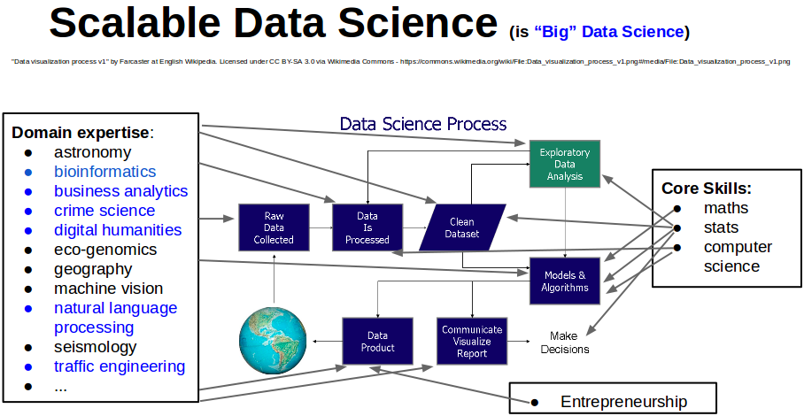
in order to understand the probabilistic models and statistical inference procedures as well implement computer programs for processing raw data - a crucial distinguishing joint skillset of a data scientist.
We will steer clear of academic/philosophical discussions on "what is data science?" and focus instead on the core skillset in mathematics, statistics and computing that is expected in a typical data science job today.
showURL("https://en.wikipedia.org/wiki/Data_science")
This course consists of
We will start with basics of programming in BASH and a review of Python before recollecting concepts in probability and setting the stage for applied statistics, including, hypothesis testing and parameter estimation.
Ethical implications
As Data scientists, you have the responsibility to ask questions such as: what is the cost of such sophisticated prediction algorithms on our society and planet? when we engage in the so-called data science process.
Here, your first assigned reading is from the following work:
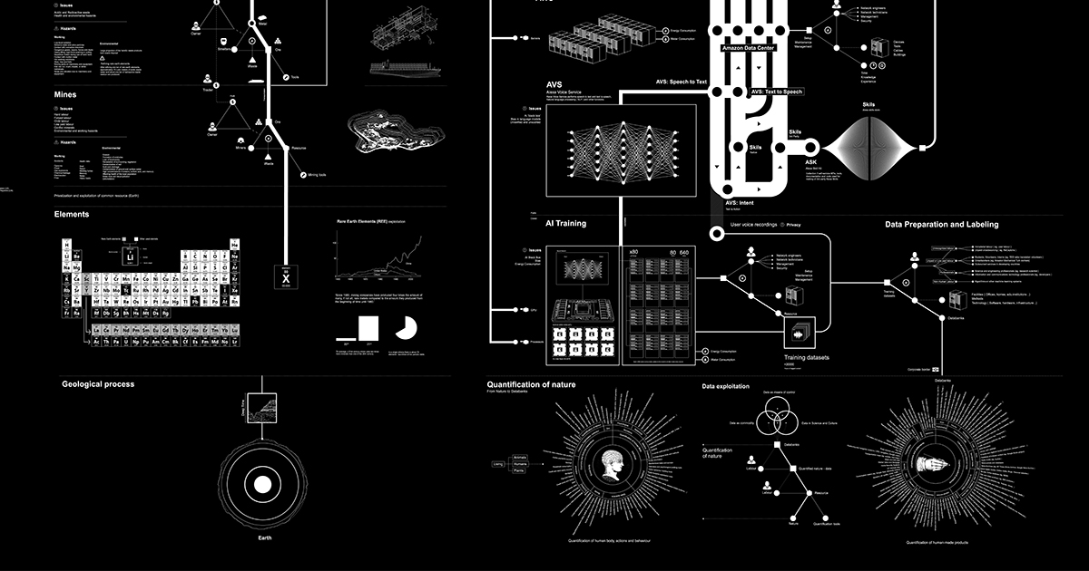
The Amazon Echo as an anatomical map of human labor, data and planetary resources. Read the 16 pages of ai-anatomy-publication.pdf with highly detailed ai-anatomy-map.pdf to complete the first problem in Assignment 1.